Transshipment Problem
Ship prescribed amounts of a commodity from specified origins to specified destinations through a concrete transportation network.
Sources- nodes with a supply of a commodity
Sinks- nodes with a demand for a commodity
Intermediate Nodes- nodes which are not a source or a sink
Definitions
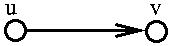
A directed graph (network) D consists of a set V(D) of vertices (also called nodes) and a set E(D) of arcs where each arc is associated with an ordered pair (u, v) of vertices from V.
Arc e= (u, v):
Transshipment Problems
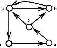
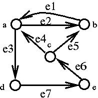
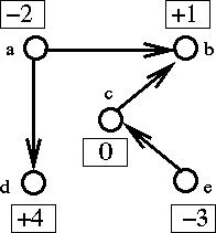
Example:
| Node | Status | Type |
|---|---|---|
| a | supply of 2 units | source |
| b | demand for 1 unit | sink |
| c | no supply or demand | intermediate node |
| d | demand for 4 units | sink |
| e | supply of 3 units | source |

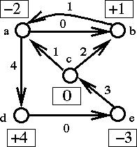
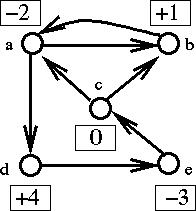
The demands are shown in the boxes.
Sources have negative demands equal to
-1 * (# units available).
Assumption: total supply = total demand.
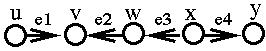
Schedule: specifies amount shipped from node i to node j along each arc.
The following schedule is ambiguous:
However, it is assumed that units are interchangeable so the trajectory of individual units is irrelevant.
Let f+(v) = the number of units entering node v
Let f-(v) = the number of units leaving node v
Conservation of flow means:
In addition, it only makes sense if the amounts shipped along each are are non-negative.
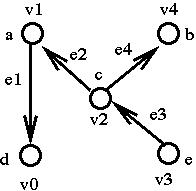
Let A be a matrix whose rows correspond to the nodes of the network and whose columns correspond to the arcs. For each arc ei= (vj, vk):
Matrix A: Incidence Matrix of the Network
      e1  e2  e3  e4  e5  e6  e7
a  [  +1  -1  -1  +1   0   0   0 ]
b  [  -1  +1   0   0  +1   0   0 ]
c  [   0   0   0  -1  -1  +0   0 ]
d  [   0   0  +1   0   0   0  -1 ]
e  [   0   0   0   0   0  -1  +1 ]
The X vector for this problem has one variable for each of the m arcs of the graph.
X= [X1 X2 X3 ... Xm]T where m= the number of arcs.
Note: This deviates from our standard convention for the use of variable m. We do this because for a digraph, n is conventionally the number of nodes, and m is the number of arcs.
Requirements
We must have A x = b where x >= 0, and
      e1  e2  e3  e4  e5  e6  e7
a  [  +1  -1  -1  +1   0   0   0 ] [X1] = [-2]
b  [  -1  +1   0   0  +1   0   0 ] [X2]   [ 1]
c  [   0   0   0  -1  -1  +0   0 ] [X3]   [ 0]
d  [   0   0  +1   0   0   0  -1 ] [X4]   [ 4]
e  [   0   0   0   0   0  -1  +1 ] [X5]   [-3]
                                   [X6]
X >= 0                             [X7]
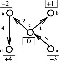
The schedule:
---------->
corresponds to:
      e1  e2  e3  e4  e5  e6  e7
a  [  +1  -1  -1  +1   0   0   0 ] [ 1] = [-2]
b  [  -1  +1   0   0  +1   0   0 ] [ 0]   [ 1]
c  [   0   0   0  -1  -1  +0   0 ] [ 4]   [ 0]
d  [   0   0  +1   0   0   0  -1 ] [ 1]   [ 4]
e  [   0   0   0   0   0  -1  +1 ] [ 2]   [-3]
                                   [ 3]
                                   [ 0]
Let cij be the cost of shipping one unit from i to j along arc (i, j).
The cost of a schedule is cT * x.
Find the cheapest schedule.
The LP:    Minimize  cT * x

subject to    A x = b, x >= 0.
A Transshipment Problem is formulated as above where A is the incidence matrix of some network, and the sum of the entries of b is zero (the total supply equals the total demand).
Note that the sum of the n equations is zero:
e1 e2 e3 e4 e5 e6 e7 a [ +1 -1 -1 +1 0 0 0 ] [X1] = [-2] b [ -1 +1 0 0 +1 0 0 ] [X2] [ 1] c [ 0 0 0 -1 -1 +0 0 ] [X3] [ 0] d [ 0 0 +1 0 0 0 -1 ] [X4] [ 4] e [ 0 0 0 0 0 -1 +1 ] [X5] [-3] [X6] [X7]so A x = b reads as 0=0. Remove the last equation to get rid of the dependence:A* x = b: e1 e2 e3 e4 e5 e6 e7 a [ +1 -1 -1 +1 0 0 0 ] [X1] = [-2] b [ -1 +1 0 0 +1 0 0 ] [X2] [ 1] c [ 0 0 0 -1 -1 +0 0 ] [X3] [ 0] d [ 0 0 +1 0 0 0 -1 ] [X4] [ 4] [X5] [X6] [X7]Matrix A* is called the truncated incidence matrix
Notes 6.1: Page 12.Graph Theory Definitions
A (undirected) path of length k-1 is an alternating sequence of nodes and arcs of the form:
v1, e1, v2, e2, v3, e3, ..., vk-1, ek-1, vk
where ei= (vi, vi+1) or (vi+1, vi) is an arc of the network.
A (undirected) cycle of size k is an alternating sequence of nodes and arcs of the form:
v1, e1, v2, e2, v3, e3, ..., vk-1, ek-1, vk ek, vk+1
where ei= (vi, vi+1) or (vi+1, vi) is an arc of the network and vk+1 = v1.
Notes 6.1: Page 13.A network is connected if there is a path between every pair of nodes.
A network is acyclic if there are no cycles.
A tree is a connected, acyclic network.
A subgraph H of network D is a directed graph such that V(H) is a subset of V(D) and E(H) is a subset of E(D).
A subgraph H is a spanning subgraph of D if V(H) = V(D).
A spanning tree of network D is a spanning subgraph of D that is a tree.
Notes 6.1: Page 14.Trees and Feasible Solutions
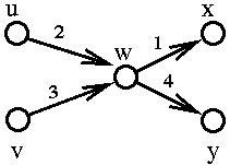
The following picture shows a feasible solution associated with a tree:
Not all trees correspond to feasible solutions. Consider for example:
Notes 6.1: Page 15.Labeling the Tree
Pick any node of T and label it v0.
Use BFS (breadth first search) to number the other nodes by v1, v2, ..., vn-1 and to number the arcs of the tree by e1, e2, ..., en-1.
Let B be the truncated incidence matrix for T with the row corresponding to v0 deleted.
e1 e2 e3 e4 v1 [ -1 +1 0 0 ] v2 [ 0 -1 +1 -1 ] v3 [ 0 0 -1 0 ] v4 [ 0 0 0 +1 ]The matrix B is upper triangular.
The diagonal has +1/-1 entries so B has full rank.Conclusion: B x* = b* has a unique solution (the * means delete the row which corresponds to v0).
Notes 6.1: Page 16.The Network Simplex Method considers only feasible solutions that correspond to trees.
We saw before: the dual variables have an economic interpretation.
Here, interpret yi to be the cost of one unit of the commodity at node i.
If one unit is bought at node i and then shipped along arc (i, j) of cost cij to node j, then the fair price at node j is yi + cij.
If the cost of doing this is less than the current cost of the commodity at node j, it pays to ship along arc (i,j).
If the cost of doing this is more than the current cost of the commodity at node j, it pays to not ship along arc (i,j).
Notes 6.1: Page 17.The Network Simplex Method
Step 1: Assume the price of the commodity at v0 is 0 and use the current feasible tree solution to determine fair prices at all the other nodes.
Note: there are n-1 equations and n unknowns so the fair prices are not unique. If y is a solution, then so is the vector obtained by adding a constant d to each entry of y. We arbitrarily set y0=0 to get a unique solution.
Step 2: Look for an arc not in T where it pays to buy and ship. If there are none- stop, the solution is optimal.
Step 3: Update the tree solution.
The new arc forms a cycle with T. Assume t units are shipped along that arc. Traverse the cycle in the direction that corresponds to the new arc adding or subtracting t from the amount shipped on each other arc to ensure conservation of flow.Find the maximum value of t so that none of the shipped amounts are negative. The new arc is added and an arc whose shipped amount is decreased to zero is deleted.
Notes 6.1: Page 18.
Later: what should we do if we have no initial feasible tree solution?